Excel Use Formula to Determine Which Column to Look at
Let us first see the exact match. If you are sure that you only have numeric values in your column your data start from row 1 and your data range in continuous you can.
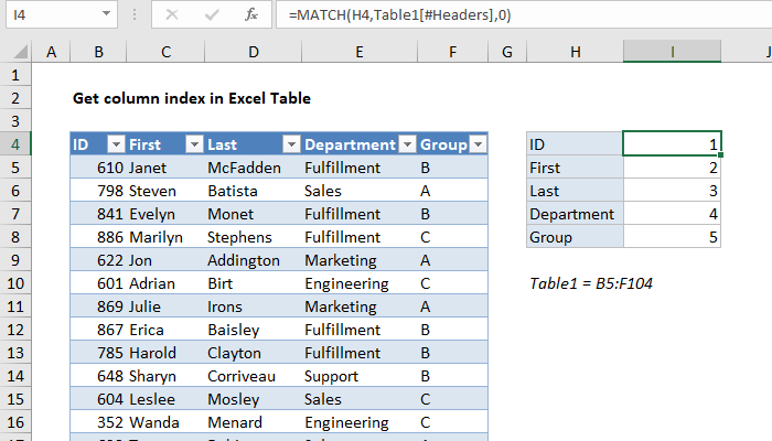
Excel Formula Get Column Index In Excel Table Exceljet
It is quite easy to figure out the row number or column number if you know a cells address.
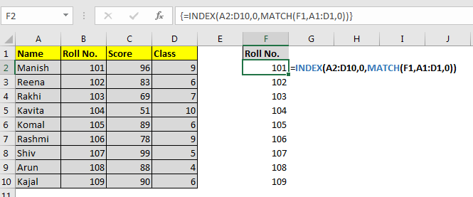
. Using the formula above we can get the last column that is in a range with a formula based on the COLUMN function. SUMIFSINDEXtbl_invMATCHC7tbl_invHeaders0INDEXtbl_invMATCHB7tbl_invHeaders0B8 where we use INDEXMATCH arguments for both the first sum_range argument and the second criteria_range argument. The formula you would enter is.
You can run the function without it. We want to look up the salary of James Clark not James Smith not James Anderson. The MATCH function returns the position of a value in a given range.
You can use the COLUMN function to quickly determine the col_index_num of the VLOOKUP formula without having to count columns. Type in the value you wish to find. Using the VLOOKUP Formula to Lookup Value in Column and Return Value of Another Column.
Insert the MATCH function shown below. Two-way lookup with formulas. Drag the formula down to the other cells in column C clicking and dragging the little icon on the bottom-right of C2.
Instead you could use a formula using a combination of SUMPRODUCT INDEX and ROW functions such as this one. Insert the formula in NOT ISERROR MATCH A2B2B10010 the formula bar. Press Enter to assign the formula to C2.
In the cell you want to place the lookup value select one formula from below. The formula used is MINCOLUMNA3C5COLUMNSA3C5-1. Excel will match the entries in column A with the ones in column B.
Copy this formula into the D column. To lookup and return the sum of a column you can use the a formula based on the INDEX MATCH and SUM functions. In the cell F1 you need to enter the second.
INDEXC3C13SUMPRODUCTB3B13C16D3D13C18ROWC3C130 You use the SUMPRODUCT function to find out the row where both criteria are met and return the. This is the lookup_vector for the LOOKUP FunctionIn our case the lookup_value is 2 but the largest value in the lookup_vector is 1 so the LOOKUP Function will match the last 1 in the array and return the corresponding value in the result_vector. In our formula this is the trickiest part.
And you can get the column with the formula of Column NK60. And the other returns the position of the second dash. The new formula would look something like this.
Specifies the number of characters you want to return. With no reference the function returns the column of the cell that contains the formula. LOOKUPLookup_ValueLookup_VectorResult_Vector The following formula finds Marys age in the sample worksheet.
You use two FIND or SEARCH functions one determines the position of the first dash. Click Find All to find all the instances of the value in the worksheet. 1 Your data needs to be set up in a table in this example the table name is Data1 2 The table needs to.
When you include this reference the function returns the column number of the specified cell. The syntax of the COLUMN function COLUMNreference Theres only a single argument reference. If the cell address is NK60 it shows the row number is 60.
Furthermore there is another similar type of formula formed using the VLOOKUP function. VLOOKUPA2Data1COLUMNData1Location0 There are a few conditions. See the example below.
The Formula for the COLUMN function is as follows. Continue to click Find Next to move through all the available values in the Worksheet. Heres what this formula does.
There are two types of VLOOKUP formulas. Excel functions formula charts formatting creating excel dashboard others. Start Your Free Excel Course.
To join strings use the operator. The LOOKUP function finds a value in a single row or column and matches it with a value in the same position in a different row or column. In the Ribbon select Home Editing Find Select.
Heres the result youll see. This example teaches you how to perform a two-column lookup in Excel. To confirm after entering the formula you need to press the combination of keys CTRL SHIFT Enter as this formula will be executed in the array.
When we give a single cell as a reference the COLUMN function will return the column number for that particular reference. The following is an example of LOOKUP formula syntax. Orange LOOKUP575 A2A6 B2B6.
It is the cell or a range of cells for which we want the column number s. In your workbook press CtrlF on the keyboard. You need to click CTRL SHIFT Enter for confirmation again.
And the curly braces will appear in the function ROW. List the column and row headers you want to look up at see screenshot. Formula LOOKUP419 A2A6 B2B6 Looks up 419 in column A and returns the value from column B that is in the same row.
Reference is any cell reference. Of course you can get the row number with formula of Row NK60. To lookup the intersection of a given row and column you need to follow below steps.
SUMINDEX C5F110MATCH I6 C4F40. In the example shown the formula in I7 is. One gives the exact match of the lookup value and the other gives a partial match.
The COLUMN function asks for only one argument that is the reference.
How To Lookup Entire Column In Excel Using Index Match

Excel Formula Lookup Entire Column Exceljet
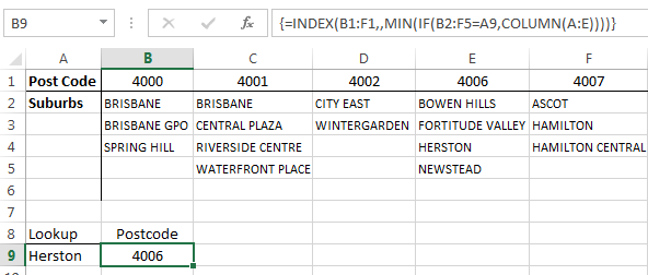
Excel Find Column Containing A Value My Online Training Hub
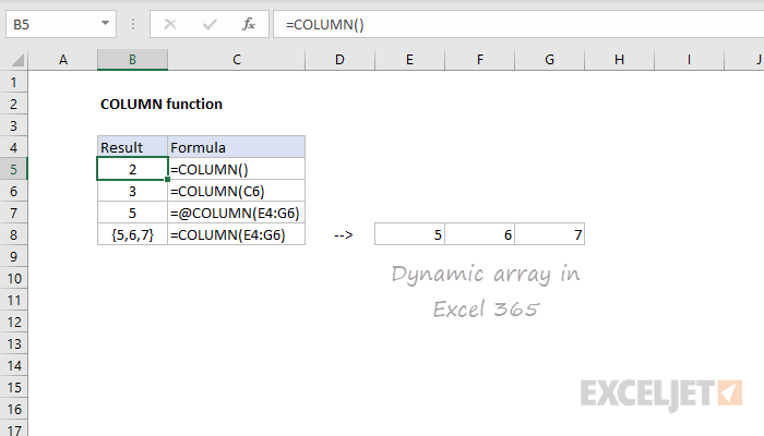
How To Use The Excel Column Function Exceljet
Belum ada Komentar untuk "Excel Use Formula to Determine Which Column to Look at"
Posting Komentar